A Visual Primer on Regression Isolation via Bisection

Identifying regressions via bisection is one of those software debugging techniques that I find under utilized and under appreciated in the software industry.  Bisection can be used to isolate changes in anything from BIOS updates to software updates to source code changes.  This article provides a backgrounder on what bisection is, and how it is useful in identifying points where a regression has been introduced.

This is the first in a set of three posts covering regressions.

Bisection Method in Mathematics

Wikipedia defines the Bisection Method as follows.

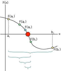
The bisection method in mathematics, is a root-finding method which repeatedly bisects an interval then selects a sub-interval in which a root must lie for further processing. It is a very simple and robust method, but it is also relatively slow. Because of this, it is often used to obtain a rough approximation to a solution which is then used as a starting point for more rapidly converging methods.The method is also called the binary search method and is similar to the computer science Binary Search, where the range of possible solutions is halved each iteration.

With a matching diagram as shown below.

As can be seen, it is a method of determining the root (zero crossing) of a continuous function.  Its mechanism is to bisect (divide into two equal parts) to determine over which half the root resides.  Once the side containing the root been determined, the same bisection process is repeated.  After a number of iterations, alternate root finding methods are generally more efficient.  For example, if you have a function with values of x ranging from 0 to 1 and your root crossing value is 0.500000001, you will spend a lot of time approaching that number (0.5,0.75,0.625,etc).

 Bisection Method Applied to Software

Moving to the software domain moves from a continuous approximation to a function with discrete steps.  This allows us to move from a method of approximation to an efficient and consistent method of finding a particular solution. Let us take the continuous function above, and allow that to be some function that represents either the number of tests that pass or a convenient benchmark.

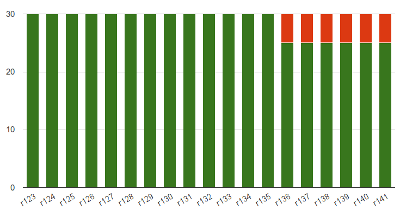
For example consider a change in the passing tests as shown below

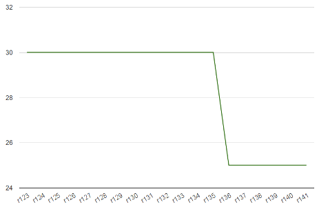
Now we can convert that into a line graph similar to

The similarity to the mathematical bisection method shown in Dake’s diagram above should be clear.  With that basis, we can apply the same root finding process.

Fortunately with software, we have discrete units of builds or checkins rather than a continuous function.  In mathematics, bisection is an approximation method – you incrementally get closer to the crossing point.  For discrete units, when the accuracy of your estimate becomes less than your discrete interval, you have found the two discrete units that represent the crossover point.  In the diagram above, you we can see that this transition occurs between r135 and r136.

A Word on Software Regressions

Let’s explore the terms regression and regression testing for a moment.  IEEE defines regression testing as follows.

Selective retesting of a system or component to verify that modifications have not caused unintended effects and that the system or component still complies with its specified requirements.

I agree with this statement, and it is one of the few definitions that points to a regression as being any unintended change.  This allow regressions to be interpreted as both negative and positive, or detrimental or beneficial.  The beneficial regressions could be an increase in tests passing, or an increase in performance of a system.   On first pass a beneficial regression might seem great, the system is working better or faster.  However the unexpected part of the definition changes our interpretation completely.

An unexpected change in system behavior implies that the developer either does not understand the system, or something else has broken which has exposed the beneficial change elsewhere.  This is typically in the case of beneficial performance regression, whereby a sudden increase in performance usually implies that some of the work has accidentally been avoided.

What You’ll Need

To determine a regression via bisection, you need the following:

1. A repeatable and deterministic test – Obviously if you can’t reliably determine if a particular build exhibits a particular behaviour, then you will be unable to track down the issue in code.
2. An ordered list of code checkins or builds – Just like the bisection method uses a continuous variable x above, your checkins or builds need to be ordered as well.  The choice of builds vs checkins is driven by both the availability of builds (everyone has a big archive of old builds from the application of Continuous Integration (CI), don’t they), and the length of time to prepare the system under test from source.    I’ll use the term build, checkin and configuration interchangeably below.

Using Bisection on Software Regressions

For tests that we have a history of execution, bisection doesn’t really help. You already have  the information, you can just look up in the results.  Bisection rules the space where you either have no previous results or some incomplete coverage in your results.

I haven’t seen the definition for the equivalent to the mathematical “root” or “zero crossing” for software regressions, so I’ll call it the Regression Fulcrum.  This is the pivot point around which we want to determine a change in behaviour. So let’s step through this with the same imaginary test above, but imagine that we do not have the intermediate information.  Declaring an explicit value also allows tests that exhibit an inherent variability to be identified.

First step is to determine the first result, the last result and the fulcrum.  In this case, we have a good result of 30 (units of performance, or tests passing) for r123, and 25 for r141.

We split the difference between the two builds, and look at the value for r132.  We get the value at r132 as 30.  A key assumption in bisection is that there is only one crossing point.  Hence we assume that between r123 and r132 all the builds were also good at value 30.  Note that the fulcrum comes in at 27.5 by splitting the difference between the two values.  For functional tests, this can be automatically determined, for performance tests, you would usually have a baseline performance number as the fulcrum.

We again split the difference between the r132 and r141 to r136.  Again assuming consistency between builds either side of the fulcrum, we incrementally get closer.  We know that the regression occurred between r132 and r136.

We continue this process until we have an identified the two builds that lie either side of the fulcrum.

Hence we can see that the regression was brought in by the changes introduced with r136.  You can now dig into the change and debug at that point.  It is usually a bug in that code that escaped the developers testing.

Of course the same technique can be used when you introduce a new test that is failing with the current code, but you believe was working on older versions of the code.

Scalability & Overlaps

As can be seen by the data points on the graph, to deduce the shape of the graph and hence determine when the Regression Fulcrum is crossed, you only need to run 6 tests for the data above.  We skipped 13 builds by assuming consistency either side of the fulcrum.  In fact, the efficiency of the of the numbers is O(log n). For small sets of builds, the benefits of bisecting regressions carries some overhead, depending on the changes between the two known regression points.  The value however increases exponentially as the number of builds increases.

Software has a particularly bad way of devolving nearly instantly.  You have the build broken for a couple of days, and you get a couple of regressions.  You have a regression in the code for a couple of days, and you get more regressions.  To handle layered regressions in this way, you have to include patches, fixes or other changes as a secondary setup in preparing for the next data point in your regression.  CI and aggressively isolating regressions are your best medicine to keeping your code clean.

Follow Up Articles

I trust that if you made it this far into the article, you got some value out of it.  Look for two more articles in this series over the next week.

Questions, comments and suggestions below.